Tipping Points in the Earth’s Climate System
Modern climate science tells us that increased emissions of greenhouse gases, most notably carbon dioxide, will change the climate that we are used to and have consequences for ecosystems and societies worldwide. A rise of just several degrees can have large and widespread impacts that dramatically alter civilization, but there are worries aside from a slow and steady rise. Climatic records show that large, widespread, and abrupt climate changes have occurred repeatedly in the past. Dr. Richard Alley of Penn State University has lectured on this topic and has used an analogy of the climate being like a drunken college student– when you don’t do much to it then it will just sit there, but if you move it around a little bit then it will stagger about and maybe fall. The last ten thousand years or so (the Holocene) has been an unusual time of relative calmness, with little variation in the climate. However, for most of the last 100,000 years, and even before, this has not been the case. One of the potential threats that comes from altering the chemistry of the atmosphere, and changing the land around to suit or needs, is the ability to flip a “climate switch” and force it between different states. Other possibilities include crossing critical thresholds, such as melting the arctic sea ice, that will have large socio-economic and/or ecological consequences. Such events have been labeled “tipping points” and many scientists (notably James Hansen of NASA, Alley, and others) have started to issue many warmings that the Earth may not respond to a new climate is a nice and steady fashion.
A formal definition of a tipping point is given in Lenton et al., 2008 and will be used here–
…the term ‘‘tipping element’’ to describe subsystems of the Earth system that are at least subcontinental in scale and can be switched—under certain circumstances—into a qualitatively different state by small perturbations. The tipping point is the corresponding critical point—in forcing and a feature of the system—at which the future state of the system is qualitatively altered.
Earlier definitions, such as that of the National Academies of Sciences in their report on abrupt climate change defined abrupt change as happening “when the climate system is forced to cross some threshold, triggering a transition to a new state at a rate determined by the climate system itself and faster than the cause.’’ In other words, the response is nonlinear. In Alley et al (2003) the authors used an example of leaning slightly over the side of a canoe causing only a small tilt, but leaning just slightly more will cause the canoe to tip over, and you fall into the lake.
When people think of a “tipping point” the scenario of the movie “The Day After Tomorrow” where the world plummets into a huge global freeze in days may come to mind. Notwithstanding the thermodynamic impossibilities of this scenario, what might actually happen is a climate that is simply less stable than today and “flickers” back and forth between states on timescales of years to decades. Such a scenario would make adaptation difficult. In that sense, you might not just talk about a climate change but the level of climate variability. To illustrate the difference, consider this graph
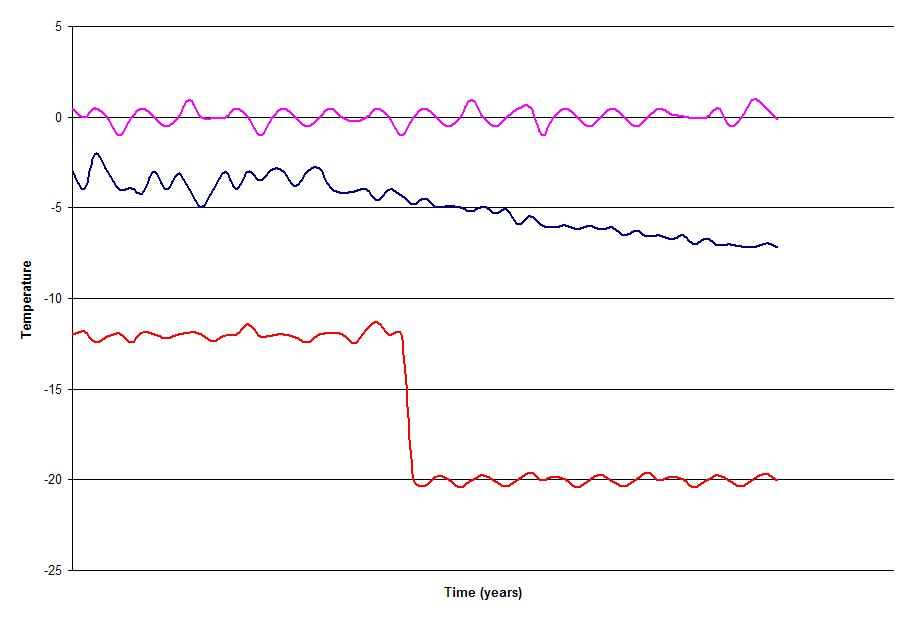
Curve “a” (top) looks like a typical set of meteorological observations; this could be a series of annual temperatures, snowfall, or some other variable. Let the time be over a few hundred years. Curve “a” shows a stationary series (i.e., the average value remains pretty much constant). The level of variability is the fluctuation about the mean, and all three series have some small degree of variability, but differing degrees of climate change– the top series has no climate change, the second has a gradual trend toward cooling, while the third shows the level of variability with some sudden drop in temperature during the record, but the average temperature remaining pretty much constant before and after the shift. None of these need be the case…the next figure shows implications of a more variable climate:

In the first curve, the climate remains effectively constant while the amplitude of variability more than doubles over the period of observation. The second curve is a more probable scenario in the real world, where the degree of variability changes as the climate cools. For a long time-series you can construct distributions to visualize the number or frequency of observations over the data range. For instance, if temperatures have been randomly sampled over a climatological time period and there is no longer any warming or cooling trend, and if the variability remains constant, then the frequency distribution should look bell-shaped. A good example might be this,

If the climate were to warm by a few degrees, then the simplest manifestation from this change would be a shift in the mean of the distribution. However, many researchers also believe that a shift to a warmer climate would lead to more variability, and so the standard deviation would rise and you get a greater spread of temperatures about the new mean.
A few “tipping points” (there are others not here) that are presented in Lenton et al (2008) and will be discussed below include, with timescales– Melting of Arctic sea-ice (in decades), decay of the Greenland ice sheet (over a few hundred years), collapse of the Atlantic thermohaline circulation (maybe 100-200 years), increase in the El Nino Southern Oscillation (around 100 years), and substantial decline of the Amazon forest (around 50 years). Pictorially, you can see the differing tipping points in this paper, but in general changes in one will have global effects, and probably large ones. –

Lenton et al (2008)
Changes in North Atlantic Circulation
Climate records over the last 110,000 years and beyond are dominated by large and abrupt changes with millennial spacing, many of which occurred on yearly to decadal timescales. Records show warming since the ice age staggered back to cold conditions several times, with one especially prominent reversal called the Younger Dryas, after a small arctic plant that was an indicator of arctic tundra conditions. Glacial to interglacial changes are paced by orbital variations (called Milankovitch Cycles) with the eccentricity and obliquity factors notably prevalent. Last warm interglacial approximately 130,000 years ago and is called marine isotope stage (MIS) 5e, the Eemian, or the Sangamonian in North America. The cooling into the most recent ice age (depending on intellectual and cultural heritage is referred to as Wisconsinan, Devensian, Weichselian, Wurm, and others) (Alley 2007). The last ice age peaked at the Last Glacial Maximum (LGM) about 18,000 radiocarbon years before present, or about 22,000 calendar years BP. Our present day warm temperatures are in a warm interglacial, the Holocene. During major glacials, sea level dropped 80-100 meters below present values. The last Ice Age contains much more noise and is characterized by substantially more variability than the modern times. Isotopic records show more than 20 interstadials (not interglacials) which have become known as Dansgaard/Oeschger (D-O) events after the scientists who identified them (Dansgaard & Oeschger, 1989). The events typically start with an abrupt warming of Greenland by some 5-10 degrees over a few decades or less (not this much over the global average!!). The warming is followed by a gradual cooling over a few hundred years, and may end with an abrupt reduction in temperature back to cold (stadial) conditions. During stadial events, cold and relatively short-lived Heinrich events occur, and represent the most extreme glacial conditions. Heinrich events are characterized by mass dumping of sediment into the North Atlantic and are marked by decreases in sea surface temperature, salinity, and plaktonic foraminifera growth. The bundling of D-O oscillations bounded by Heinrich events is called a Bond cycle.

Alley, 2007

The last 100,000 years was highly variable. During the Hengelo interstadial between 38 and 36 kya for instance, the climate across Northern Europe became warm enough that deciduous forests spread into France and coniferous forests grew into Russia (Burroughs, Climate Change in Prehistory). The deglacial warming from the LGM into the Holocene was interrupted by the Older Dryas (Heinrich event H1), then start of the Bolling-Allerod warmth (kind of a false start to the Holocene), then cooling into the Younger Dryas (sometimes called H0), until we finally hit the Holocene which kept permanent warmer and wetter conditions into present day.
The Younger Dryas (YD) is a well studied time period and represents the last significant abrupt climate change. There is little evidence it was associated with the surge of icebergs like other Heinrich events, but rather the huge release of glacial meltwater from North America. The transition into the Preboreal, the PB/YD transition, and the YD/Holocene transition were pretty fast.

Ocean water sinks when it becomes dense. The addition of salt increases the density of water at constant temperature. The colder and saltier the water, the more dense it will become. Because the North Atlantic exhibits these qualities, the water of the North Atlantic propel a “conveyer belt” (see Broeker) of ocean circulation that, as a consequence, drives heat from the tropics up along the east coast of North America, and into the higher latitudes. The warm surface water that moves toward Europe is the “Gulf Stream” and the warm air over the Gulf Stream (the atmospheric component) is called the “Nordic Heat Pump.” Warm, low-salinity water flows north along the surface of the Atlantic becoming saltier. Cooling of the saltier water produces high enough densities for it to sink and flow southward in the deep oceans and other ocean basins. The term “thermohaline circulation” refers to the density-driven movement of water around the world’s ocean basins, with density determined by the water’s temperature and salinity (Rahmstorf 2006).
A shutoff in North Atlantic Deep Water formation and the THC can occur if sufficient freshwater or heat enters the North Atlantic to halt the density-driven North Atlantic Deep Water formation. In terms of climate, it matters whether the polar ocean water sinks before it freezes, or freezes before it sinks. A shutdown of the THC could bring cooler temperatures to the mid to high latitudes. The 8.2 Ka event (cooling roughly 8200 years before present) was a result of the brief reorganization of the North Atlantic circulation. With the retreat of ice due to the Holocene warmth, significant volumes of freshwater were released into the North Atlantic and Arctic. The 8.2k event was caused by an outburst flood from Lake Agassiz which drained tremendous amounts of water into Hudson Bay very rapidly (Clarke et al., 2004).
It is harder to get a THC shutdown today as the Laurentide ice shelf no longer sits on Canada, and hard to keep sea ice off England in the winter even if you freshen the ocean. The IPCC has a less than 10% chance of a shutdown this century. Unfortunately, we do not yet have the knowledge to quantify the fresh water influx to get a shutdown. In such a scenario, the radiative forcing from CO2 would still likely cause a warming effect even to places in the Northern Hemisphere, and there would certainly be no catastrophic ice age as in the “Day After Tomorrow” movie, however there will probably be large regional changes, and different consequences for different areas.
Thresholds, Stochastic Resonance
Large and abrupt changes between different modes of the North Atlantic seemed to have occurred over a distribution of ~1500 years in the past. Because our dating is uncertain by a few percent, it is hard to tell with high confidence if this is just a “preferred spacing” or a true periodicity at 1500 years. One possible mechanism by which “noise” and a very weak “signal” (a weak but true 1500 year periodicity in forcing) could combine is presented in Alley et al., 2001. Systems with a weak periodic signal may combine with other signals (e.g., white noise) to cause mode switches. For example, the orbital variations causing ice ages appear to be too small on its own to lock the planet into a glacial state. Two other things must happen– first, the amplitude of the orbital cycle must be amplified, and some threshold must be crossed which locks the climate system into an ice age through positive feedback (or stochastic resonance). A resonating system is where some low frequency is amplified until it dominates the system (click on graph for better quality).

The threshold drawn on this diagram represents a global temperature where positive feedback is triggered– and the system may reach this point when randomness is superimposed upon peaks in the underlying cycle. Clustering of a bunch of events above the threshold can lock the climate system into a new state. Stochastic resonance says that a long-period (even weak) cycle can force warming if that cycle is superimposed upon by noise and a threshold exists which lock the system into a new state.
ENSO variability
During La Nina, winds blow westward across the pacific and accumulate warm water off the coast of Australia. The El Nino part of the cycle features weakening of the tropical winds, warm water flowing eastward, releasing humidity into the atmosphere bringing floods into Peru. Cooler water is upwelling back north which evaporates less efficiently than warm water, and Australia and areas of Asia experience drought-like conditions. The El Nino Southern Oscillation is the most significant ocean-atmosphere mode and has worldwide implications for climate. It is influenced by the meridional temperature gradient across the equator, thermocline depth, and East Equatorial Pacific thermocline sharpness. A deepening of the thermocline from increased ocean heat uptake could result in more frequent El ninos. Corals, ocean sediments, and other records indicate that the mid-Holocene had dampened ENSO variability with a transition toward a strong regime in the past few thousand years (Moy et al., 2002; McGregor and Gagan, 2004). During the warm early Pliocene (~4.5 to 3.0 million years ago), the most recent interval with a climate a few degrees warmer than today the average west-to-east SST gradient was similar to El Nino like conditions today, and that period may have exhibited permanent El Nino like conditions (Wara et al., 2005).
AMAZON
The Amazon rainforest occupies around 5.8 million square kilometers (IPCC 2007 WG2), and carries around one third of the planet’s biodiversity (fromhere). The Amazon, like many forests worldwide are threatened very much by global warming, and because of their socio-economic, ecological, and aesthetic value are of major concern as far as impacts go. Over the last three decades, over 600,000 square kilometers have been lost to deforestation in just Brazil, another large anthropogenic-induced threat. Losses of forest bring higher temperatures, longer dry seasons, and substantially reduced precipitation to this very large region. The Amazon would also respond heavily to changes in ENSO that were to occur in a warmer climate. Simulations, like those of a recent paper by Cook and Vizy show that the Amazon could decline by 70% by the end of the century under emission scenarios that involve little change from present courses. In this simulation, much of the rainforest in the central Amazon north of about 15°S is replaced by savanna vegetation, and other areas by grassland. The surface energy budget will respond heavily with changes in temperature, loss of the overhead canopy, evaporation changes, etc. In addition, mass releases of CO2 will occur; rainfall, carbon in soil, and carbon stored in vegetation will all likely decline by 50-75% by 2100, and much of the area may become desert (Cox et al., 2004; Betts et al., 2004).
Ice
Summer sea ice in the Arctic is expected to be gone as soon as the middle of this century. Both summer and winter Arctic sea-ice are going through area coverage that is declining at present (faster in the summer) (Stroeve et al., 2007). This has implications for the ice-albedo feedback which allows the darker ocean to absorb more sunlight that the highly reflective sea ice, ecological consequences, ocean circulation implications, as well as vegetation changes. Loss of seasonal ice represents the most rapid of climate change responses. Abrupt retreat occurs when ocean heat transport to the Arctic increases rapidly.
The Greenland Ice Sheet (GIS) and Western Antarctic Ice Sheet (WAIS) will not be lost in decades, but could possibly be lost on timescales of a few hundred years. Each of them has the potential to raise sea level by around 23 feet. The IPCC and others show increased melting and accelerated ice flow around the edges of GIS in the past couple of decades. If you have no melting on top, the ice at the shelf edge, then a bit of warming may do nothing; if you have the ice almost too warm, and warming causes a bit of thinning that lowers the surface and warms more, there is a threshold beyond which the ice sheet cannot survive, so the effect of a little warming is expected to be larger if the temperature before the warming is higher. From Lenton et al (2008) again:
In some simulations with the GIS removed, summer melting prevents its reestablishment, indicating bistability, although others disagree. Regardless of whether there is bistability, in deglaciation, warming at the periphery lowers ice altitude, increasing surface temperature and causing a positive feedback that is expected to exhibit a critical threshold beyond which there is ongoing net mass loss and the GIS shrinks radically or eventually disappears. During the last interglacial (the Eemian), there was a 4- to 6-m higher sea level that must have come from Greenland and/or Antarctica.
Changes in Greenland are now fast, and even the IPCC 2007 report neglects contributions from accelerated glacial flow from the edges. WAIS is currently declining rapidly, and further concerns arose from the acceleration of glaciers that fed the Larsen B ice shelf after its collapse several years ago. Most of the WAIS is grounded below sea level, and collapse may be triggered by the intrusion of warming ocean water beneath or by surface melting. WAIS could also respond to global warming projections by the end of the century, but like the Greenland Ice Sheet, would probably take a couple hundred years for large changes in sea level and collapse.
Abrupt Climate Change. R. B. Alley, J. Marotzke, W. D. Nordhaus, J. T. Overpeck, D. M. Peteet, R. A. Pielke, Jr., R. T. Pierrehumbert, P. B. Rhines, T. F. Stocker, L. D. Talley, and J. M. Wallace (28 March 2003). Science 299 (5615), 2005. DOI: 10.1126/science.1081056
Clarke, G. K. C., D.W. Leverington, J. T. Teller, and A. S. Dyke. 2004. Paleohydraulics of the last outburst flood from glacial Lake Agassiz and the 8,200 BP cold event. Quaternary Science Reviews, 23, 389-407
Cook, K.H., E.K. Vizy. 2007. Effects of the 21st Century Climate Change on the Amazon Rainforest. Journal of Climate
Dansgaard, W., and H. Oeschger, 1989: Past environmental long-term records from the Arctic. The Environmental Record in Glaciers and Ice Sheets, H. Oeschger and C. C. Langway Jr., Eds., Wiley, 287–318.
McGregor and Gagan, Western Pacific coral δ18O records of anomalous Holocene variability in the El Niño–Southern Oscillation. Geophysical Research Letters, Vol. 31, L11204, doi:10.1029/2004GL019972, 2004
Moy, C.M., G.O. Seltzer, D.T. Rodbell, and D.M. Anderson, 2002: Variability of El Nino/Southern Oscillation activity at millennial timescales during the Holocene epoch. Nature, 420, 162-165
Permanent El Niño-Like Conditions During the Pliocene Warm Period. Michael W. Wara, Ana Christina Ravelo, and Margaret L. Delaney (29 July 2005) Science 309 (5735), 758. DOI: 10.1126/science.1112596
P.M. Cox et al., “Amazonian Forest Dieback under Climate-Carbon cycle Projections for the Twenty-First Century,” Theoretical Applied Climatology 78 (2004): 137-156
R.A. Betts et al., “The Role of Ecosystem-Atmospheric Interactions in Simulated Amazonian Precipitation Decrease and Forest Dieback under Global Climate Warming,” Theoretical Applied Climatology 78 (2004): 157-175
S. Rahmstorf: Thermohaline Ocean Circulation. In: Encyclopedia of Quaternary
Sciences, Edited by S. A. Elias. Elsevier, Amsterdam 2006.
Sciences, Edited by S. A. Elias. Elsevier, Amsterdam 2006.
Stochastic Resonance in the North Atlantic. Richard B. Alley, S. Anandakrishan, P. Jung (April 2001) Paleooceanography, Vol. 16, No. 2, 190-198
Stroeve J., M. M. Holland, W. Meier, T. Scambos, M. Serreze (2007), Arctic sea ice decline: Faster than forecast, Geophys. Res. Lett., 34, L09501, doi:10.1029/2007GL029703.
Timothy M. Lenton, Hermann Held, Elmar Kriegler, Jim W. Hall, Wolfgang Lucht, Stefan Rahmstorf, and Hans Joachim Schellnhuber. Inaugural Article: Tipping elements in the Earth’s climate system. Proceedings of the National Academy of Sciences 105: 1786-1793; 10.1073/pnas.0705414105
Wally Was Right: Predictive Ability of the North Atlantic “Conveyor Belt” Hypothesis for Abrupt Climate Change. Richard B. Alley., Annu. Rev. Earth Planet. Sci. 2007. 35: 241–272
RECENT COMMENTS
John Baez on Retirement Bob Armstrong on Retirement Martin Lewitt on Judith Curry on ‘dogma… Ross on Physics of the Greenhouse Effe… John Brookes on Judith Curry on ‘dogma…
No comments:
Post a Comment